Excel Lookup Function Published June 6th, 2019 down to video
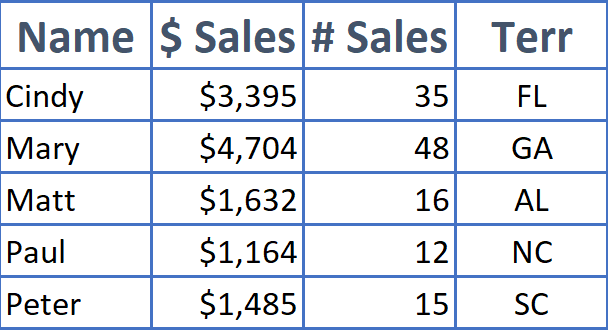
Today's article is about Excel's Lookup function. Imagine, from the data below, that you wished to be able to pull Mary's sales units. The Lookup function can help!

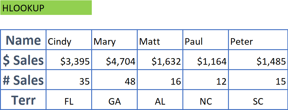
There are 2 versions of the lookup function... vlookup (for vertical data - columns) and hlookup (for horizontal data - rows). Use vlookup if the data is in columns, hlookup if the data is in rows as below:

Whether you are using vlookup or hlookup there will be 3 or 4 parameters that you need to set; lookup_value, table_array, col_index_num and, optionally, range_lookup.
lookup_value - This is the value that you wish to find. The "subject" of the function.
table_array - This is the range of data that makes up the table that you will search. Note that the lookup_value must be in the first column of the table_array data, or the first row if using hlookup.
col_index_num - Once the lookup_value is found* this is the column cell that will be returned. * see the final parameter.
range_lookup - Setting range_lookup to False means to look for an exact match only. Setting range_lookup to True, or omitting this parameter, means to find an approximation. When looking for an approximation the function will start at the top of the list and look for a value greater than the lookup_value. Once found the function will move up one row and return the corresponding value in column col_index_num.
In the example of VLOOKUP(F3,A4:D9,3,FALSE) we are looking for F3 in the data range of A4:D9 and returning the value in column 3. Since the fourth parameter is set to False we are looking for an exact match. Since we are using vlookup we know that our data is in columns (vertical). This also means that the value in F3 needs to be in column A since we are looking from A4 through D9. The A in A4 means that column A is the first column of data.
Using the data below, if F3 was equal to Mary then we'd return a 48 as 48 is in the 3rd column of the row that contains Mary.

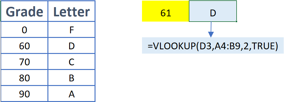
Let's look at an example when the last parameter, range_lookup, is omitted or set to True. In this case the function will look for the first value that is greater than our lookup_value (61 in this case) starting from the top of the column. 70 is the first element greater than 61. So the function moves back one row and returns the 2nd element which is a D. For best results you'll want the data sorted by the first column... the column containing the lookup_value.
